Mt. Eden Computer Applications 1
 Excel Warm-Up 8
How to Calculate Your Grade Point Average (GPA)Your grade point average (GPA) is calculated by dividing the total amount of Grade Points earned by the total amount of Class Units attempted. Your grade point average may range from 0.0 to a 4.0. A = 4.00 grade points WF/F=0 grade points P/NP (Pass/No Pass) courses are not factored in the student's GPA |
INSTRUCTIONS:
In Excel open a this workbook: My Transcript.
Insert a new row to the top of your worksheet.
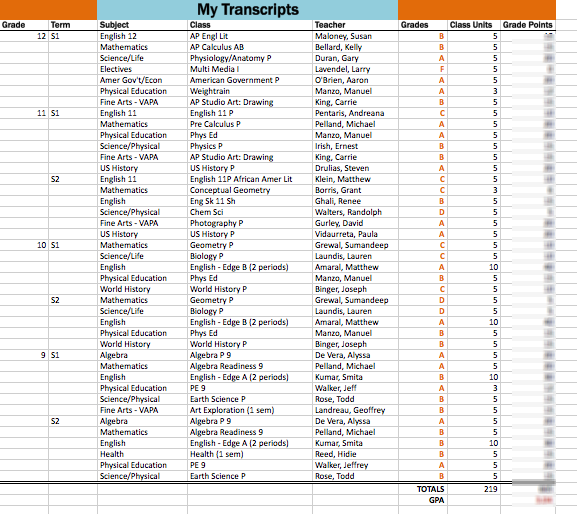
In D1 type "My Transcript" set the type to Franklin Gothic Bold and 22 points.
Select cells D1 through F1 and merge and center them. Color in that merged cell Aqua, Accent 5, Lighter 40%. Color cells A1 to C1 and G1 to I1 Orange, Accent 6, Darker 25%.
In cell I2 type "Grade Points". Set all of the labels to Franklin Gothic Bold and 14 points.
Set all of the grades in (the text in) column G to Bold, Right Justified and Orange, Accent 6, Darker 25%.
We will use these simple grade point values (no +s or -s):
A = 4.00 grade points If you want to add the +s and -s you can. Use the numbers at the beginning of the warm-up and add the IF tests for the +s and -s to the formula below. To assign the proper grade points to it we need to convert the grade in column G to a number and multiply it by the number of class units (the *H3). |
In cell I3 type this formula:
=IF(G3="A", 4, IF(G3="B", 3, IF(G3="C", 2, IF(G3="D", 1, 0))))*H3
Distribute drag the formulas from the I3 to I43.
In G44 type "TOTALS" set the type to Bold and Right Justified.
In G45 type "GPA" set the type to Bold and Right Justified.
Put the Total Class Units in cell H44, that is the SUM of the column H3 to H43.
Put the Total Grade Points in cell I44, that is the SUM of the column I3 to I43.
Put the GPA in cell I45, that is the Total Grade Points divided by the Total Class Units.
In the Home tab, Number group reduce the number of decimal places to two: 3.04.
Make the number Bold and Red Accent 2, Darker 25%.
Make a border to the under cells A2 through I2.
Make a Double Border to the under of cells A43 through I43.
In A45 type your name.
In A46 type your period number.
Done!
WHEN YOU ARE DONE...
Save your completed file in your folder in your Documents folder on your computer.
TURN IN THE COMPLETED FILE THROUGH GOOGLE CLASSROM.
~~ This is worth 10 Participation points.~~
Back to Apps1 Main: CLICK HERE.