Mt. Eden Computer Applications 1

Excel Warm-Up 7

INSTRUCTIONS:

In Excel open a this workbook:
Women & Women First Books.

Select cells A2 through J5.

Create a 2-D Clustered Column Chart.

To make the x axis measure the months instead of the book type: in the chart tab under Data, click Switch Plot.

In the Chart Design tab:

1. Add the horizontal axis label "Month" and the rotated vertical axis "Sales in dollars".
2. Add the Chart Title (Title Above Chart) "Women & Women First Books: Quarterly Sales".

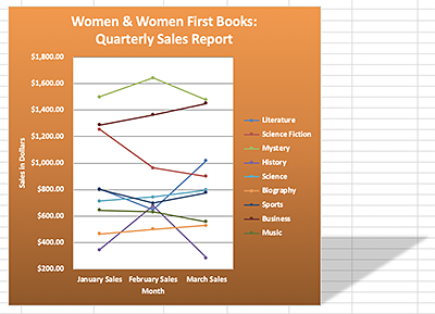Change Chart Type to 2-D Line with Markers.

In the Chart Design tab:

Set Quick Layout to the Layout 1.

In the Chart Format tab:

1. Set the Shape Fill to the Orange, Accent 6 and then the Gradient to Dark Variation Linear Up.
2. With Shape Effects set the shadow behind the chart to Perspective: Upper Right.
3. Click on the horizontal grid lines to select them and color them with the Shape Outline:
   Black, Text 1, Lighter 50%.
4. Click between the horizontal grid lines and with the Shape Fill: White.

Click to select the entire chart again and set all of the text to White, Bold and to 11 point size.

Set the title to 20 points.

Scale the chart so that it is a similar proportion to the example shown above and so that it is easy to read, then place it below the data.

In A16 type your name.

In A17 type your period number.

Done!

WHEN YOU ARE DONE...

Save your completed file in your folder in your Documents folder on your computer.

TURN IN THE COMPLETED FILE THROUGH GOOGLE CLASSROM.

~~ This is worth 10 Participation points.~~

Back to Apps1 Main: CLICK HERE.